Predictive Price Modeling for Airbnb listings

The project aims at predicting the price of an Airbnb listing given a number of features. The project involved exploratory data analysis, data pre-processing, feature selection, Model Fitting, Model Comparison and deploying the containerised Webapp on AWS using CI/CD Pipeline.

What is the goal of the project ?

The Short Answer: Assisting Airbnb hosts to set appropriate price for their listings

The Problem: Currently there is no convenient way for a new Airbnb host to decide the price of his or her listing. New hosts must often rely on the price of neighbouring listings when deciding on the price of their own listing.

The Solution: A Predictive Price Modelling tool whereby a new host can enter all the relevant details such as location of the listing, listing properties, available amenities etc and the Machine Learning Model will suggest the Price for the listing. The Model would have previously been trained on similar data from already existing Airbnb listings.
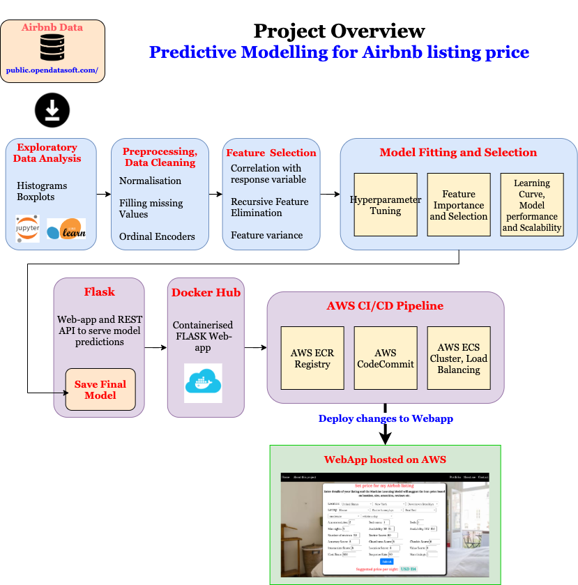
Project Overview

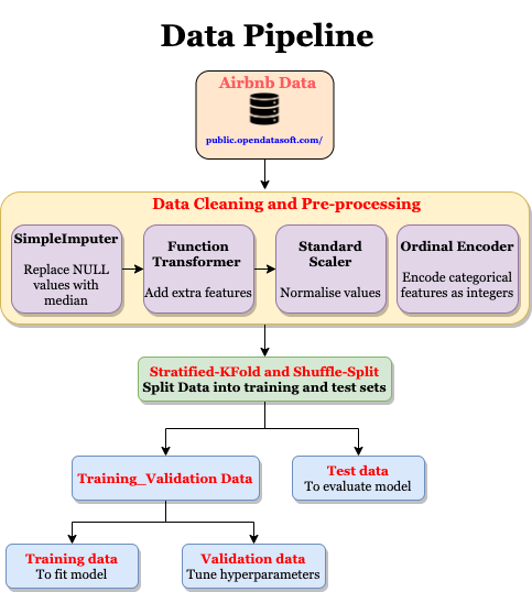
The project involved the following steps,

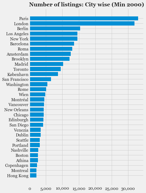
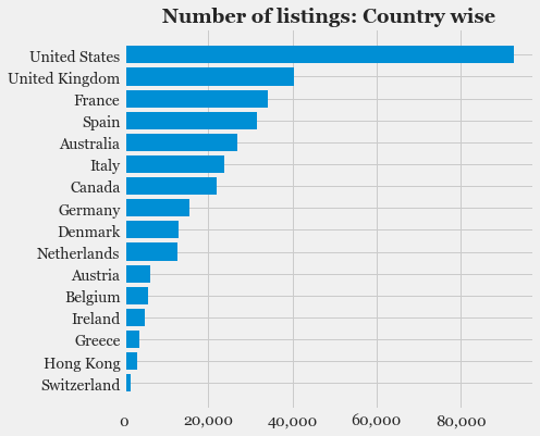
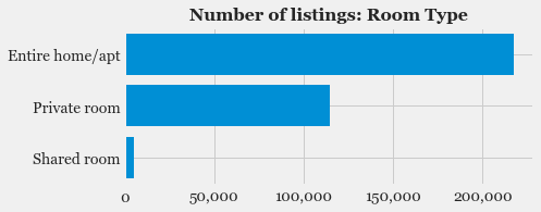
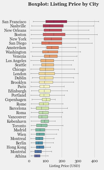
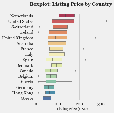
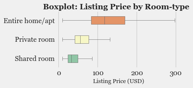
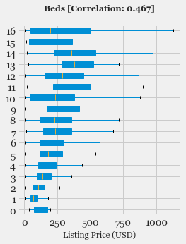
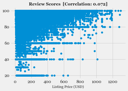
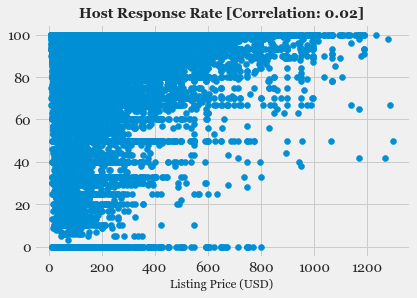
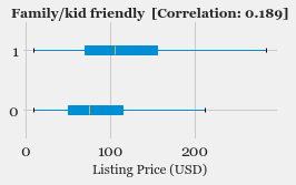
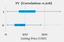
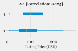
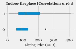
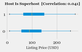
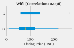
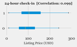
  • Exploratory Data Analysis: Explore the various features, their distributions using Histograms and Box-plots
  • Pre-processing and Data Cleaning: Normalisation, filling missing values, encoding categorical values
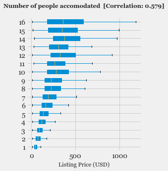
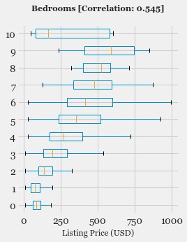
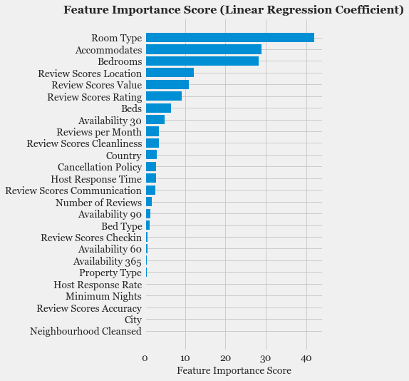
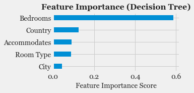
  • Feature Selection: Study the correlation with response variable (Listing Price) and determine which features are most useful in predicting the price.
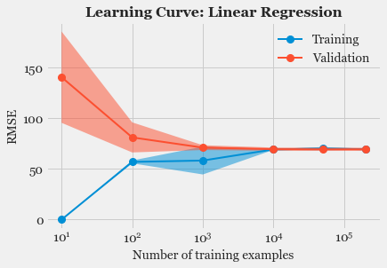
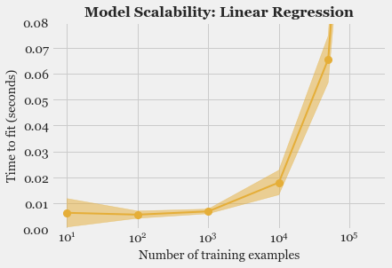
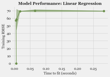
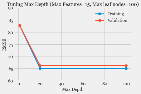
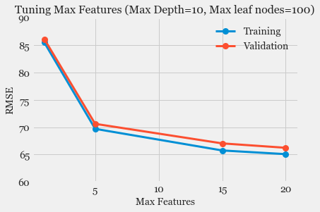
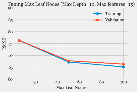
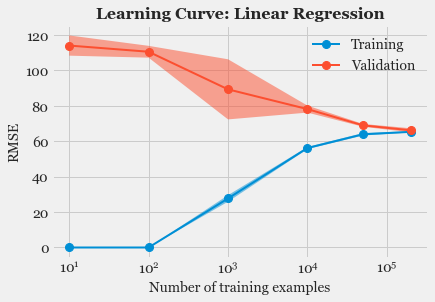
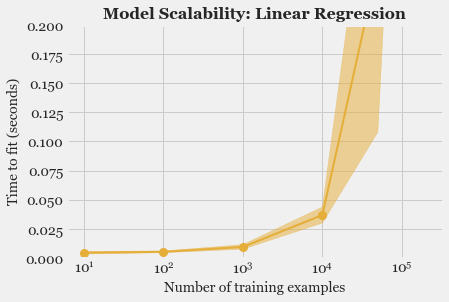
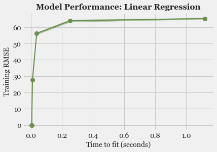
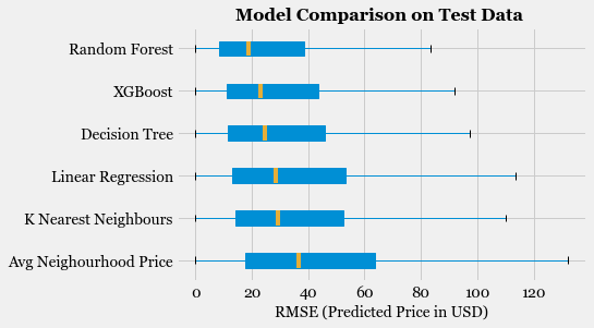
  • Model Fitting and Selection: Training different models, tuning hyper-parameters and studying Model performance using Learning Curve.
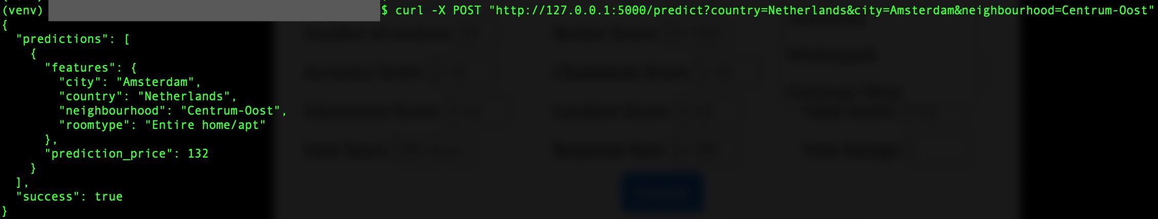
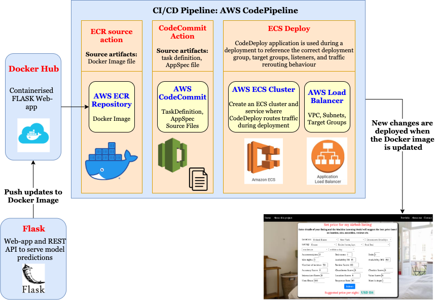
  • Model Serving: Using FLASK to deploy and serve Model predictions using REST API
  • Container: Using Docker to containerise the Web Application
  • Production: Using AWS CI/CD Pipeline for continuous integration and deployment.

End Result

The screen capture of the entire application in use is shown below. Users can enter all the relevant details of their listings, the trained Predictive Model will then predict and return the price of the listing given all the features. The Webapp can be explored here.

About Dataset

The Dataset used in this project was obtained from public.opendatasoft.com. There are a total of 494,954 records each of which contains details of one Airbnb listing. The total size of dataset is 1.89 GB.

The dataset has a large number of features which can be categorised into following types,

  • Location related: Country, City, Neighbourhood
  • Property related: Property Type, Room Type, Accommodates, Bedrooms, Beds, Bed Type, Cancellation Policy, Minimum Nights
  • Booking Availability: Availability 30, Availability 60, Availability 90, Availability 365
  • Reviews related: Number of Reviews, Reviews per Month, Review Scores Rating, Review Scores Accuracy, Review Scores Cleanliness, Review Scores Checkin, Review Scores Communication, Review Scores Location, Review Scores Value
  • Host related: Host Since, Host Response Time, Host Response Rate, Calculated host listings count, Host Since Days, Host Has Profile Pic, Host Identity Verified, Is Location Exact, Instant Bookable, Host Is Superhost, Require Guest Phone Verification, Require Guest Profile Picture, Requires License
  • Amenities: TV, Wireless Internet, Kitchen, Heating, Family/kid friendly, Washer, Smoke detector, Fire extinguisher, Essentials, Cable TV, Internet, Dryer, First aid kit, Safety card, Shampoo, Hangers, Laptop friendly workspace, Air conditioning, Breakfast, Free parking on premises, Elevator in building, Buzzer/wireless intercom, Hair dryer, Private living room, Iron, Wheelchair accessible, Hot tub, Carbon monoxide detector, 24-hour check-in, Pets live on this property, Dog(s), Gym, Lock on bedroom door, Private entrance, Indoor fireplace, Smoking allowed, Pets allowed, Cat(s), Self Check-In, Doorman Entry, Suitable for events, Pool, Lockbox, Bathtub, Room-darkening shades, Game console, Doorman, High chair, Pack ’n Play/travel crib, Keypad, Other pet(s), Smartlock

The price of the listing will serve as labels for the regression task. The goal of this project would be to predict these price of the listings.

Exploratory Analysis

To get a better insight into where the listings are located, the number of listings in various cities and countries are plotted in the figure below. In the given dataset, United States has the most number of listings followed by European countries and Australia. In terms of cities, Paris, London, New York, Berlin, Los Angeles are some of the cities with most number of listings.

Airbnb offers three types of listings,

  • Entire home/apartment
  • Private Room
  • Shared Room
Entire home is by far the most popular type of listing offered followed by Private Rooms and then a small share of the total listings are shared rooms.

Intuitively it is reasonable to expect that the listing location and the listing property type are two of the most important factors in determining the price of the listing. The following plots shows the distribution of listing prices across various cities and the difference in price amongst the three property types.

Few noticeable observations from the above plots,

  • Netherlands, US, Switzerland, Ireland, UK have amongst the highest average listing price.
  • In terms of cities, 10 of the top 12 cities with the highest average listing price are in the US. Clearly Airbnb listings are more expensive in the US compared to other European cities.
  • As expected, the cities with the highest listing prices are all major tourist attractions. Outside of the US, Amsterdam and Venice are the cities with highest average listing price.
  • As expected, Entire homes have the highest prices followed by Private Room and then Shared Rooms.

Feature Engineering: What features will be useful in predicting the listing price ?

Although the dataset consists of large number of features for listings, not all of them will help in predicting the listing price. In fact, different features will have different influences in .Feature Engineering refers to selecting a subset of features or adding new features which will aid in better prediction of the response variable which is the Listing Price in this project.

The following figures show the distribution of various features against the listing price. This will aid in determining which features are correlated with the listing price and can thereby result in the Models making better predictions.

As expected, the most important factors that determine the price of a listing are Number of people accommodated, Number of bedrooms, Number of beds, all of which have a Pearson's Correlation Factor of more about 0.45 with the Listing Price. Amenities like TV, AC also show a slight positive correlation. But it is clear that there are no hidden features which plays a major role in determining the listing price, bigger the home/apartment with more bedrooms and beds, higher is the listing price.

Data pre-processing and cleaning

Before feeding these features as input to the Machine Learning Model, the data will need to be pre-processed and cleaned. The following block diagram shows the Data Pipeline with the operations involved in pre-processing and data splitting.

Data Pre-processing

The pre-processing operations involved are listed in the following table.

Name Feature Type Operation
Imputer Numerical Replace NULL values with Median
Standard Scaler Numerical Standardise input data to have 0 mean and unit variance
Ordinal Encoder Categorical Encode discrete values into integers

The following code snippet shows the pre-processing pipeline implemented using the Python library Scikit learn.

After pre-processing, the dataset is divided into 3 splits the details of which are listed in the following table.

Data Purpose Split Ratio Number of Samples
Training To fit Model 0.8 270,058
Validation To tune hyperparameters 0.1 33,757
Test To evaluate model performance 0.1 33,757

Modeling: Training Machine learning models, Model Selection

Model Evaluation Metric

Since this is a Regression task (predicting the price of listing), various evaluation metrics such as Variance Explained Score, Mean Absolute Error, R2-score, RMSE (Root Mean Squared Error) can be used. In this project, RMSE is used to evaluate and compare different Machine Learning Models.

Regression Models

The following Regression Models were explored in this project,

  • Baseline Models
    • Average Neighbourhood Price
    • K-Nearest Neighbours Regression
  • Linear Regression
  • Decision Tree Regression
  • Random Forest Regression
  • XGBoost Regression

Baseline Models

Before trying various Machine Learning Models, it is important to set baseline performances based on simple heuristics or simple models. Accordingly the following two models were used as baseline to compare the other Machine Learning Models.

  • Average Neighbourhood Price: Estimate the listing price to be the average price of all the listings in the neighbourhood.
  • K-Nearest Neighbours Regression: As defined , the target is predicted by local interpolation of the targets associated of the k-nearest neighbors in the training set.

Linear Regression

As defined here, LinearRegression fits a linear model to minimize the residual sum of squares between the observed targets in the dataset, and the targets predicted by the linear approximation.

Linear Regression: Feature Importance

The Importance of features as determined by the Linear Regression coefficients is shown in the following plot. As expected Room Type, Number of people accommodated and Number of bedrooms are the most important features in determining the price of the listing.

Linear Regression: Model Learning, Performance and Stability

The following code snippet shows how Scikit Learn's learning_curve method can be used to study the Model learning, performance and stability.

The learning, performance and stability for the Linear Regression Model are shown in the following figures. Learning curve shows how the Model predictions improve as it sees more training examples. The fact that the training and validation RMSE converge to similar value, shows that the Model is not overfitting.

Model scalability can be studied by plotting the time it takes to fit the Model as the number of training examples increases. The Model performance can be examined by plotting the Model Evaluation Metric (RMSE) against the time it takes to fit the Model. Together these curves will be very useful in comparing various Models and selecting a final Model for predictions.

Decision Tree Regressor

Decision Tree Regressor: Feature Importance

The following figure shows the Top5 features sorted by the Feature Importance as determined by the Decision Tree Regressor. As expected, the number of bedrooms, people accommodated, room type and location of the listing (country, city) are the most important features in determining the listing price.

Decision Tree Regressor: Hyper-parameter tuning

In order to get the best possible results from any Model, it is vital to determine the right combination of hyper-parameters to be used. This process is known as hyper-parameter tuning. It involves training the Model with different values for a set of parameters. The Model performance is then computed using the Validation Dataset. The parameter combination which yields the best performance is the one that will eventually be selected while comparing various Models. The code snippet to do this using Grid Search and Randomized Search Cross Validation is shown here,

To determine the best possible values, the following different values of parameters were tried using Grid Search Cross Validation.

Hyper-parameter Values
Maximum Depth [1, 20, 100]
Maximum Number of Features [1, 5, 15, 20]
Maximum number of leaf nodes [5, 50, 100]

The best estimator for was determined to be with the following values of hyper-parameters, Max Depth=20 , Max Features=20 and Max Leaf Nodes=100.

Decision Tree: Learning Curve, Model Scalability and Performance

Model Evaluation and Comparison

The final step of Model Selection is to compare the Prediction RMSE of all the tuned classifiers on Test Dataset. In this step, it is important to consider not just the Mean or Median RMSE, instead consider the entire range of RMSE obtained over different samples in the Test Dataset or over different splits of Cross Validation Data. The box plots of RMSE on Test Data for different Regression Models are shown in the following plot,

It can be observed that amongst the Models considered here, Random Forest seems to be the one with the lowest Median RMSE, also with the lowest IQR (Inter-Quartile Range). The Median RMSE error for Random Forest is less than 20 USD, so the Model is successful to a large extent in predicting the price of the listing.

Deployment, Serving and Production: CI/CD Pipeline

Model deployment using FLASK Application

A FLASK Webapp is developed in order to serve the Model Predictions and showcase the capabilities of the project. The following code block shows how the model is used to get inference for a given input image.

Serving Model Predictions: REST API as Web Service

The Model predictions can also be served as a Web Service by using REST API. The following code snippet shows how this can be accomplished. The model output is returned as a JSON object.

The following figure shows how the Model predictions can be obtained using the above REST API.

Model in Production: FLASK, Docker, AWS CI/CD Pipeline

The production pipeline consists of the following components,

  • FLASK Webapp: Webapp and REST API to serve Model Predictions
  • Docker: Containerised FLASK Webapp which can then be deployed in any environment
  • AWS: CI/CD Pipeline
    • ECR Repository: The Docker Image is stored in this repository. Any changes to this image will trigger changes in the rest of the pipeline and the updates to the image will then be deployed to the Web Application.
    • CodeCommit : The pipeline is configured to use a source location where the following two files are stored,
      • Amazon ECS Task Definition file: The task definition file lists Docker image name, container name, Amazon ECS service name, and load balancer configuration.
      • CodeDeploy AppSpec file: This specifies the name of the Amazon ECS task definition file, the name of the updated application's container, and the container port where CodeDeploy reroutes production traffic.
    • CodeDeploy: Used during deployment to reference the correct deployment group, target groups, listeners and traffic rerouting behaviour. CodeDeploy uses a listener to reroute traffic to the port of the updated container specified in the AppSpec file
      • ECS Cluster: Cluster where CodeDeploy routes traffic during deployment
      • Load Balancer: The load balancer uses a VPC with two public subnets in different Availability Zones.

Resources